The content on this page has been converted from PDF to HTML format using an artificial intelligence (AI) tool as part of our ongoing efforts to improve accessibility and usability of our publications. Note:

No human verification has been conducted of the converted content.
While we strive for accuracy errors or omissions may exist.
This content is provided for informational purposes only and should not be relied upon as a definitive or authoritative source.
For the official and verified version of the publication, refer to the original PDF document.

If you identify any inaccuracies or have concerns about the content, please contact us at [email protected].

AS TM1 Accumulation Rates – Technical Analysis as at 31 August 2021

1. Context and scope

1.1Actuarial Standard Technical Memorandum 1: Statutory Money Purchase Illustrations ("AS TM1") specifies the assumptions and methods to be used for the calculation of statutory illustrations of money purchase pensions (also known as defined contribution ("DC") pensions) for annual SMPI statements.

1.2Department of Work and Pensions (“DWP”) has proposed that pension schemes sending data to dashboards will be required to supply an estimated retirement income (“ERI”) alongside other data elements. Under DWP's proposals, money purchase schemes will also be required to include the projected pot size (known as “ERI pot") used to calculate the ERI, if this is held. This means that a user logging on to a dashboard would be able to see their projected ERI for all schemes and a final projected pot value for their money purchase schemes, where schemes hold it. The current proposal is for money purchase schemes to use the methodology and assumptions for AS TM1 to project both the ERI and the ERI pot data elements.

1.3In February 2022, the FRC published a consultation paper to propose amendments to AS TM1. The amendments proposed were intended to produce more consistent, comparable results across different DC schemes and hence make the projections more suitable for a dashboard environment. One key proposed change to AS TM1 is in relation to the accumulation rates assumptions. This consultation concluded in May 2022. This paper is issued alongside publication of the AS TM1 v5.0.

Scope

1.4This paper has been prepared by the FRC to provide further details of the technical analysis carried out to support our proposals in the consultation in 2022 in relation to the accumulation rate assumptions, covering:

Data used within our analysis;
The relationship between past volatility and future returns;
How the proposed volatility groups were determined; and
How the proposed accumulation rates by volatility group were determined.

1.5This paper is not intended to examine or compare alternative approaches for determining accumulation rates, such as using rates based on asset classes, or a single fixed rate. It is also not intended to discuss the practical implications of applying this approach or obtaining necessary data. The rationale and impact analysis of the proposed changes to the accumulation rate assumptions are set out in the consultation paper and the subsequent feedback statement and impact assessment published alongside AS TM1 v5.0.

1.6We recommend this paper to be read in conjunction with the consultation paper, feedback statement and impact assessment and the finalised version of AS TM1 v5.0.

1.7The technical analysis described in this paper was completed before the release of the consultation paper in February 2022. It was based on data up to 31 August 2021, and our understanding of market conditions up to early February 2022, This paper does not include any update to the analysis to account for any subsequent developments. The FRC intends to conduct similar but separate analyses on updated data in advance of the implementation of AS TM1 v5.0, and for subsequent reviews.

1.8The FRC would like to thank Dr Paul Cox for his insights and expertise on this work.

2. Overview

Overview of methodology to determine the accumulation rate assumptions

2.1As set out in the consultation paper, in developing the methodology to determine the accumulation rate assumptions, we observed the following principles:

The resulting accumulation rate assumption can be considered reasonable given observed data in the market.
The resulting accumulation rate assumption should take account of additional returns that can be expected from higher-risk funds, in respect of a fundamental assumption of capital market theory that increased risk should be correlated with increased long term average return.
The resulting accumulation rate assumption can be determined consistently for different funds.
The resulting accumulation rate assumption and the resulting statutory illustration should be easy to describe to savers and to be understood by them.
The determination of the resulting accumulation rate assumption should not place an undue burden on providers.
The methodology should not, as far as is practicable, cause or encourage unintended behaviours which are not in consumers' interests.

2.2In developing our methodology, we have considered numerous stakeholders. These included both users and providers of SMPIs and pensions dashboards ERIs, across various different types of pensions arrangements. Consideration was also given to the relative proportions of SMPIs across different types of pension arrangement. In particular, we have considered that the majority of recipients of SMPIs are invested in default strategies in large pension schemes.

2.3In developing the methodology and calibration of the accumulation rates, we conducted analysis on the following areas, drawing on research conducted externally:

The extent to which historic volatility correlates with future returns of pooled pension funds (set out in Section 4)
Rationale for choosing boundaries between volatility groups, including the volatility of various asset classes over time (set out in Section 5)
The stability of the volatility groups assigned to funds over time and potential adjustments to the methodology to address the instability of volatility groups (set out in Section 6) in order to: * increase the stability of ERI projections for individual retirement savers * reduce the burden on providers from needing to update their assumptions more frequently than necessary
What accumulation rates might be appropriate for ERI illustration calculations for each volatility group, both for the annual SMPI and for display on pensions dashboards (set out in Section 7).

2.4We conducted this analysis in conjunction with independent research commissioned from Dr Paul Cox of the University of Bath. A summary of our interpretation of Dr Cox's research is provided in Appendix 1.

3. Data used

3.1The data set used in the analysis was based on data drawn from Morningstar. This included monthly returns for 1,335 UK wholesale pooled pension funds covering the period from 31 January 1990 to 31 August 2021. The data was checked and cleaned before being provided to us, but we conducted further checks and excluded some of the data from our analysis. For example:

Some funds had missing returns for some months. For funds that remain extant, we understand that this results from the fund manager not reporting the fund's return in that month. The return reported in the following month does not include the return for the missing month. Therefore, any calculation of a volatility or a return which included a month with missing data was treated as null and excluded from the analysis. Funds with missing data were still included, but only for periods for which they had enough valid data to calculate a valid 5-year volatility and subsequent 5, 10, 15 or 20 year return.
There were a number of funds which reported 0 returns in a given month. This differs from missing returns in that it indicates that a return of 0 was actually reported. Since fund prices are discrete, some returns of exactly 0 can be expected. Instances of 0 returns were more common in funds with lower average returns, which further supports the notion that these are genuine returns.
However, some funds had long strings of 0 returns, often for a year or more, coinciding with other funds with the same provider reporting 0 returns, and/or near the beginning or end of the periods for which returns were reported. As a result, the data for periods with multiple consecutive returns of exactly 0 were treated as missing.

3.2After making the above adjustments and excluding funds without a string of at least 120 valid monthly returns (as would be needed to calculate a 5-year volatility and subsequent 5-year return), the data set was reduced from 1,335 funds to 1,075. The graph below shows the number of funds which are present at a particular date in our final data set:

Line graph showing the number of funds present at a particular date in the final data set, from 1990 to 2020. The number of funds starts low (around 200 in 1990), increases to over 1000 by 2008, and remains high, fluctuating, until 2020. The x-axis shows years from 1990 to 2020, and the y-axis shows 'No. of funds' from 0 to 1200.

3.3Dr Cox provided a taxonomy of the funds, which we used to categorise funds into broad asset categories within our analysis.

3.4The use of individual single-asset funds was useful in providing insight into the interplay between asset type and volatility. However, the vast majority of SMPI users are in invested in multi-asset funds, often comprising of combinations of the types of funds present in our data. This should be borne in mind when considering the results of our analysis, and was the reason Paul Cox's analysis focused instead on synthetic combinations of the funds present in the data.

4. Volatility as a predictor of future returns

4.1The external research indicates that there is a substantial positive correlation between the volatility group and long-term returns. We conducted our own analysis to verify this by inspecting the relationship between 5-year volatility[^1] and subsequent 10-year and 15-year real return for every fund at every month possible.

4.2The following chart shows the relationship between the 5-year volatility and the subsequent 15-year returns:

Scatter plot titled "All data points: raw volatility vs 15-year return" showing the relationship between 5-year volatility (x-axis, 0% to 35%) and 15-year real return (y-axis, -6% to 14%). Data points are clustered, generally showing a positive correlation where higher volatility corresponds to higher returns, but with significant spread.

4.3The correlation coefficients between the 5-year volatility and subsequent return were examined:

	15-year returns Pearson coefficient	15-year returns Spearman coefficient²	10-year returns Pearson coefficient	10-year returns Spearman coefficient
5-year volatility	0.64	0.61	0.50	0.48

4.4This shows that there is evidence of a substantial correlation between 5-year volatilities and subsequent returns and the results are broadly consistent with the external research. The results are consistent with our expectation that the correlation between volatility and subsequent return will generally get stronger as the time period over which returns are measured increases.

4.5We also considered the extent to which the process of dividing funds into discrete groups based on their volatility would impact this relationship. For the purposes of this analysis, we used the Synthetic Risk and Reward Indicator (“SRRI”) categorisation for Undertakings for Collective Investment in Transferable Securities (UCITS) to group the funds[^3].

4.6The correlation coefficients between the SRRI category to which the fund belongs to (based on its 5-year volatility) and subsequent return was also examined:

	15-year returns Pearson coefficient	15-year returns Spearman coefficient	10-year returns Pearson coefficient	10-year returns Spearman coefficient
5-year volatility	0.64	0.61	0.50	0.48
SRRI level	0.66	0.63	0.56	0.52

4.7The above shows that the strength of the relationship is not significantly impacted when funds are categorised into different levels such as the SRRI categories based on their volatility.

5. Volatility groups

5.1The purpose of this analysis was to establish a set of volatility groups with which a set of accumulation rate assumptions can be associated, and which allows us to meet the principles set out in paragraph 2.1. To this end, we aimed to establish a set of volatility groups which met the following principles:

Funds in the same group should be sufficiently homogenous that it is reasonable to project them with the same accumulation rate
Funds in different groups should generally be discernibly heterogeneous such that it is reasonable to project them with different accumulation rates
The group ranges should strike a balance between being sufficiently broad that funds will change between them infrequently, but retain a reasonably small step change in accumulation rate assumption between different groups
The groups should be appropriate under the prevailing market conditions at the point at which providers are required to calculate their 5-year volatilities
We should avoid spurious accuracy in drawing the boundaries between groups.

5.2The SRRI categorisation already exists as a method of dividing funds into separate risk groups based on their volatility. While this formed a natural starting point for our investigation, the SRRI categorisation was established for a different purpose, under different market conditions, and without any intention of associating different growth assumptions with the risk groups. The external research conducted by Dr Paul Cox also indicated that the 7-level SRRI risk categorisation, without adjustment, is limited in its usefulness as a proxy to expected fund returns.

Volatilities of different types of funds

5.3Using the fund classifications referred to in paragraph 3.3, we calculated various statistics on the volatilities of funds within each asset grouping. The key results as at 31 August 2021 (the latest date for which we had data) are as follows:

	Equity	Fixed income	Money Market	Multi asset	Property
95th percentile	21.0%	12.5%	5.0%	16.6%	15.2%
Mean	16.3%	10.0%	4.9%	12.9%	8.3%
Median	16.1%	9.9%	5.0%	13.2%	7.5%
5th percentile	13.0%	7.2%	5.0%	8.5%	5.4%

5.4The development of the medians over time is shown below:

Line graph showing the median 5-year volatility over time (1995-2021) for different asset classes: Equity, Multi-asset, Property, Fixed income, and Money market. Equity shows the highest volatility, fluctuating between 10% and 20%. Fixed income and Multi-asset are in the middle, and Money market shows the lowest volatility, mostly below 5%. The y-axis ranges from 0% to 25%, and the x-axis shows years from 1995 to 2021.

5.5In considering principle (b) in paragraph 5.1 above, we looked at whether there is a clear separation in the volatilities between broad asset classes, such that for instance the volatility of most funds categorised as 'equity' exceeds that funds categorised as 'fixed income'. The below chart shows the development of the various percentiles of asset classes, which we would consider relevant if attempting to separate different asset classes based on volatilities. In this chart, most equity funds lie above the green line, most fixed interest funds lie between the light and dark blue lines, and most money market funds fall below the orange line.

Line graph showing 5-year volatility percentiles (5th and 95th) for Equity, Fixed Income, and Money Market assets from 1995 to 2021. Equity 5th percentile is consistently higher than Fixed Income 95th percentile, which is higher than Money Market 95th percentile, indicating clear separation but also occasional overlaps. The y-axis ranges from 0% to 18%, and the x-axis shows years from 1995 to 2021.

Setting the volatility group boundaries

5.6The results at 31 August 2021 in particular indicate two problems with adopting the 7-level SRRI categorisation for UCITS funds:

SRRIs include 3 separate groups for funds with volatilities below 5% (0%–0.5%, 0.5%-2%, and 2%-5%). The spike in volatilities following the Covid-19 pandemic means that under 31 August 2021 conditions, there would have been almost no funds in the 0 – 0.5% and 0.5 – 2% intervals. The only funds with volatilities under 5% at 31 August 2021 were money market funds, so this level of granularity would not have met our objective of keeping the groups discernibly heterogeneous.
SRRIs also include a group for funds with volatilities over 25%. Even with the relatively high volatilities seen in 2021, there were very few that would have fallen into this group. As a result, we did not consider that the analysis required to associate an accumulation rate with this group could have been sufficiently robust.

5.7The remaining boundaries used for SRRIs (5%, 10%, and 15%) are not obviously inappropriate, but were considered independently of the SRRI framework.

5.8Although only money market funds had volatilities below 5% at 31 August 2021, there are some other funds with volatilities slightly above 5%. Historically, it has not been uncommon for the volatilities of fixed income funds to fall below 5%, with even the median volatility across the fixed income funds occasionally falling below this level. Setting the upper limit for the least volatile group much higher than 5% therefore risks conflating money market funds with riskier funds. In the absence of any compelling reason to adopt a different boundary, we therefore consider 5% an appropriate upper limit for the lower volatility group.

5.9We considered setting other boundaries so as to separate asset classes into different groups – for example, adopting boundaries at 7.5% and 12.5% would have generally resulted in separate groups for money market, fixed income, and equity funds as at 31 August 2021. However, we concluded that adopting simple 5% intervals was preferable on grounds that:

Given that most funds within the middle volatility groups are likely to consist of multiple different asset types anyway, we do not consider the separation of asset types into different volatility groups to be particularly compelling rationale
Given the significant overlap between the highest-volatility fixed income funds and the lowest-volatility equity funds in 2015-19, it would not always be possible to separate asset classes as neatly as could be done at 31 August 2021
Given the variation in funds' volatility over time, using intervals of much less than 5% would increase the frequency with which funds change group. The risk of funds changing into a non-consecutive group would also start to become significant, although this would be mitigated somewhat if the boundaries are revised each year and move roughly in line with average market changes in 5-year volatility
On the other hand, our analysis in section 7 suggests that using intervals of 5% for the volatility groups results in a difference in accumulation rates of 2%p.a. Using larger intervals would result in larger step changes between different groups, and a change of 2%p.a. to an accumulation rate would already result in a significant change to ERIs, especially for those who are still several years from retirement. Intervals of around 5% do appear to strike a reasonable balance between the frequency and the size of the accumulation rate changes we would expect from one year to the next.
Boundaries at 5%, 10% and 15% coincide with SRRI boundaries and provide a simple structure

5.10The appropriateness of the groups was also considered in the context of the accumulation rates established in section 7. In particular, the differences in historic returns achieved by funds in the different groups indicates that the groups are sufficiently heterogeneous.

5.11The analysis above relies on the data in scope and market conditions at the time of the analysis. We intend to review these volatility groups against the prevailing market conditions closer to when the changes to AS TM1 are effected, and review these regularly thereafter to ensure the calibration remains appropriate.

6. Stability of volatility groups

Nature of instability of volatility groups

6.1The volatility of any given fund will vary over time for various reasons, for example, changes in the macro-economic environment, sector or fund-specific factors, or periods of historically high or low volatility moving out of the measurement period. Changes in volatility will not necessarily result in changes in expected return and therefore it is not always desirable to reflect changes in volatility with changes in the accumulation rate assumption.

6.2It is therefore useful to consider how often and why the funds would switch between volatility groups. The following chart shows the proportion of funds which switched to a different volatility group, based on the volatility groups above (0%-5%, 5%-10%, 10%-15%, 15%+) and monthly recalculations.

Stacked bar chart showing the percentage of funds moving up or down between volatility groups monthly from 1995 to 2021. Spikes in upward movement are visible around 2000, 2008, and 2020, corresponding to market crashes, followed by downward spikes about 5 years later. The y-axis ranges from -20% to 30%, and the x-axis shows years from 1995 to 2021.

6.3Based on monthly recalculations, funds switched to a different volatility group once every 2.6 years on average.

6.4There are two main causes for changes in volatility group that we consider would be advantageous to exclude.

6.5First, changes in general market conditions may cause large numbers of funds to change volatility group simultaneously. Particularly visible in the chart above are the large numbers of upward movements caused by Covid, the 2007-8 financial crisis, and, to a lesser extent, the dot com crash. In the latter two cases, spikes in downward movements around 5 years later can be seen, as the impact of the crash drops out of the 5-year volatility calculation.

6.6It is difficult to justify a mechanical increase in the expected long-term return in these funds that is then reversed out 5 years later due to the methodology deployed. For example, equity markets have largely recovered from their March 2020 Covid-related fall; there seems to be little economic basis for continuing to apply a higher accumulation rate for the remaining 5-year period. The second significant and unwanted source of changes is the discrete nature of the intervals. This means that funds near the border between two volatility groups may be required to change category a disproportionate number of times. The chart below illustrates a particular example of a fund changing category 7 times in less than 2 years, despite relatively small changes to its 5-year volatility:

Example fund 5-year rolling volatility

Line graph showing an example fund's 5-year rolling volatility, fluctuating around 10% from January 2015 to September 2016. The line shows multiple small upward and downward movements, causing several category changes within a short period. The y-axis ranges from 9.0% to 10.4%, and the x-axis shows dates from 01/2015 to 09/2016.

Mitigation of instability of volatility groups

6.7Frequent unnecessary changes in volatility groups could potentially cause confusion for SMPI and dashboard users as their projections would change significantly as a result. It would also place a burden on providers, who would have to change the assumptions used and potentially explain the changes to the users. We have therefore considered what adjustments could be made to reduce the frequency of changes between volatility groups.

6.8The SRRI framework addresses this issue by requiring the SRRI indicator to be revised only if the volatility of the fund has fallen outside the volatility range corresponding to its previous risk category on each weekly or monthly data reference point over the preceding 4 months.

6.9We considered five methods for achieving greater stability in the volatility groups:

Different frequencies of recalculation
Volatility corridors
Time lags

Different frequencies of recalculation

6.10Different parameters in each method and various combinations of the methods were investigated. To measure their potential effectiveness, we calculated the average length of time it would have taken for a fund to move into a different group, across all funds and all dates within our data set.

6.11We analysed the impact of annual, rather than monthly recalculations in two ways:

calculating the volatilities each month, but comparing it against the volatility group 12 months, rather than 1 month, prior, in order to determine whether the fund has changed group;
only recalculating the volatility group at specific dates each year - either at 31 March or 31 December.

6.12The impact on the average number of years funds stayed in the same volatility group was similar in each of the above cases, increasing from 2.6 years for monthly recalculations to around 4.7 years for the annual methods. Based on this, we consider less frequent calculations do result in less frequent changes, but the timing of the recalculations is unlikely to make a material difference to the average frequency of switches between volatility groups. Annual recalculations would also place a lower burden on providers than monthly recalculations.

Corridor

6.13Even with an annual recalculation there would be some funds (close to the top or bottom of a volatility group) that would switch regularly based on random fluctuations.

6.14We considered introducing a corridor around the boundary of the groups which will help to remove the idiosyncratic fund movements. Applying a corridor would mean that the volatility group will not be updated until the volatility moves beyond the corridor around the boundary. For example, in applying a 0.5% corridor, a fund with an in group 3 will not be reclassified to group 4 unless the volatility exceeds 15.5%. Similarly, a fund in group 4 with decreasing volatility would not be reclassified until the volatility fell below 14.5%.

6.15The 'stickiness' is assumed to be based on the group actually assigned at the previous recalculation date, rather than the volatility at the previous recalculation date. For example, if a fund has volatility of 9.9% at the first point at which it is calculated, it would be assigned to group 2 (interval of 5% to 10%). If the volatility rose to 10.1% for the following measurement, it would remain in group 2 because of the 0.5% corridor. If the volatility then rose to 10.2% the next measurement, the fund would still be assigned to group 2, not group 3.

6.16Applying a 0.25%, 0.5% or 1.0% corridor increased the average time between switches from 4.7 years (annual recalculations without a corridor) to 5.0, 5.4. and 7.0 years respectively.

6.17While increasing the size of the corridor does stabilise the volatility categories, too large a corridor would undermine the purpose of reassigning categories to the funds.

6.18As volatilities are grouped in equal intervals (with each group apart from the highest covering a 5% range in volatilities), the corridors considered were equal both in absolute terms and relative to the size of the intervals. In principle, there may be advantage in scaling the corridors with the range of the group the fund would potentially be moving either to or from. This should be considered if and when a different set of boundaries is adopted.

Time lags

6.19The effectiveness of a time lag (as adopted by SRRI methodology) was considered, so that funds only change volatility group when they have been at the new level for a given period of time.

6.20A 6-month time lag produced a similar effect to a 0.5% volatility corridor on the overall stability, with changes on monthly recalculations occurring once every 4.6 years on average.

6.21As with a volatility corridor, this primarily impacts funds with volatilities oscillating around a border for a period, with relatively low impact on the effect of market crashes, which merely result in changes being introduced 6 months later.

6.22Using a lag has the disadvantage of delaying any genuine changes which should be captured from entering our calculations, and does not appear to have advantages over the application of a volatility corridor. If recalculations are performed annually, the use of a time lag also introduces significant extra work, as monthly recalculations would need to be performed in any case to determine whether a fund has been in a new group for long enough.

Alternative time period for volatility measurement

6.23Measuring volatility over a 10-year period (rather than 5 years) increases stability of the classification. This is to be expected because the impact of extreme events becomes less pronounced. The average years staying in the same volatility group increased from 2.6 years for a 5-year period to 4.7 years for 10-year period, which is very similar to the effect of switching from a monthly recalculation to an annual recalculation.

6.24However, this would increase the volume of data required, would lock in any idiosyncratic movements for longer periods, and a similar effect could be achieved with adjustments of the volatility ranges to allow for significant market events. Further, there is an increased probability that asset strategies might change over a 10-year period and so the more distant historic data becomes less relevant when used as a predictor of future returns.

6.25Additionally, 5 years is the standard period of measurement for volatility for UCITS funds and therefore there would need to be compelling reasons to deviate from the market standard.

Reducing the impact of large market movements

6.26Significant market events are a significant source of instability in volatility levels. As a result of the Covid-19 pandemic, for example, around 40%[^4] of UCITS funds were required to update their SRRI level. Such a crash would depress the value of equity funds (and other asset types that are strongly correlated to equity) and, if the underlying assumption is that the market would revert to a long-term average, one could argue for assumption that the return of these funds would be higher than expected in the following short to medium term period. However, such crashes would not necessarily change long-term expectations of fund returns. There is a strong theoretical argument that a fund's expected return ought to be based on its beta (volatility relative to the market) and ignore market volatility. However, separating these would complicate the calculation significantly.

6.27The impact of excluding any movements within the last 60 months which are more than 2 standard deviations from the mean was analysed, as well as the impact of ignoring the top and bottom results from the period.

6.28Both of these had a much greater impact on periods including the 2020 market crash than it did on periods including the 2007-8 crash. This is because the nature and timing of the crashes were different. In 2020, prices remained relatively stable until around 21 February, following which they fell sharply until around 20 March. A relatively stable recovery then followed. This means that almost all the effect of the crash is removed if the returns in March 2020 are ignored. 2007-8, by contrast, took place over a much longer period, with falls in value and increased volatility from mid-2007 and into 2008. Also significant is that Lehman Brothers filed for bankruptcy on 15 September 2008 and that it took about a month following this for prices to reach their lowest point – meaning the biggest continuous fall in values was spread fairly evenly over 2 separate months.

6.29This illustrates a significant difficulty with any adjustments to large market movements – the impact of the adjustments is extremely sensitive to the timing of the calculations relative to the movement. Such adjustments would introduce an element of arbitrariness into the volatility categories which would not be justified and would require more detailed analysis which may only be possible after the event.

6.30Not fully accounting for the largest movements within the historical data set when calculating the volatility would also risk skewing the results, with funds more susceptible to large market movements appearing relatively less volatile.

6.31For these reasons, we do not consider it appropriate to adjust the historical data set used in order to reduce impact of large market movements.

Other considerations

6.32Because periods of market instability affect most funds in similar ways at the same time, the rank of a fund's volatility compared with other funds appears to be relatively stable, compared to the numerical value of the volatility itself which moves up or down with significant market movements and later readjustments. It might therefore be theoretically possible to set volatility group boundaries which aims to capture funds in the group based on the fund's ranking (by volatility) compared to the population of funds.

6.33It is not practicable for providers themselves to calculate a rank of their volatility compared to all other funds. However, an approximation of this may be possible to achieve by the FRC updating the boundaries between different volatility categories to allow for significant market events.

Conclusion

6.34The above analysis is summarised in the table below:

Stabilising method applied	Description	Average of years in staying within a volatility group
Base scenario	Monthly recalculation of volatilities	2.6
Different frequencies of calculation	Recalculate volatilities on an annual rather than monthly basis	4.7
Volatility corridors (monthly recalculation)	Introduce a corridor around the boundary of a group. The category will not be updated until the volatility moves beyond the corridor around the boundary	4.1 (0.25% corridor) 4.9 (0.5% corridor) 6.6 (1.0% corridor)
Volatility corridors + annual recalculation	As above, but with risk groups recalculated annually	5.0 (0.25% corridor) 5.4 (0.5% corridor) 7.0 (1.0% corridor)
Time lag (monthly recalculation)	Introduce a time lag, so that funds only change volatility group when they have been at the new level for a given period of time	6 month lag: 4.6
Alternative time period for volatility measurement (monthly recalculation)	Measure volatility over a 10-year period, rather than 5 years	4.7
Reduce the impact of large market movements	Adjust the data to remove the impact of large market movement, eg: • exclude any movements within the last 60 months which are more than 2 standard deviations from the mean • exclude the top and bottom results from the period	Results highly sensitive to precise timing of market movements and calculations

6.35Given this analysis, we consider an annual recalculation of the volatility group with a 0.5% corridor to be appropriate.

7. Accumulation rates

Overview

7.1The determination of the appropriate accumulation rate assumption for each volatility group is a subjective process. A number of considerations were taken into account, including backward-looking data-driven analysis and judgement-based forward-looking analysis:

The average historic real return of funds in scope grouped according to their volatility categories at the beginning of each return period. This retrospective approach maintains consistency with the assumption (concluded from the earlier analyses) that historic volatility has predictive power over future returns. It also maintains an empirical consistency between the volatility ranges and the accumulation rates.
The bias introduced by limiting the analysis to the time period covered, and the weight of funds at different times within this.
Whether the composition of funds within each group in the analysis period would carry through into future.
The accumulation rate assumptions used by providers as collected in the latest AS TM1 survey, and output from various asset models in the market.
Given inherent uncertainty in predicting the future and limitations of the models and data – and that one can reduce contributions closer to retirement, but a shortfall discovered too late may be unbridgeable - whether it is appropriate to introduce a degree of prudence.

7.2It is also useful to bear in mind the context in which the accumulation rate assumptions will be used. AS TM1's methods and assumptions are used for the purpose of pension illustration, rather than an accurate individualised pension projection. We consider it important that the resulting accumulation rate assumption can be determined consistently for different funds, and the resulting statutory illustration should be easy to describe to savers and to be understood by them.

Retrospective analysis

7.3As observed in the external research, longer return periods are significantly better correlated with 5-year volatility. 5-year returns in particular are quite poorly correlated with 5-year volatilities. However, using longer periods for return calculations reduces the number of periods for which funds can produce data that can be used in the calculation. For 20-year returns, returns and volatilities could only be compared for periods starting 31 December 1994 (when a 5-year volatility can first be calculated) until 31 August 2001 (which is 20 years before final day of data in scope). This materially reduces the data set and risks biasing the results because of the relatively small period considered, and relatively few funds in the data set during earlier years.

7.4The analysis therefore focusses on the 10-year and 15-year historical returns earned by the funds. The shorter period has the benefit of a higher number of funds with sufficient data for the analysis; the longer period has the benefit of better correlation between risk and return.

7.5The analysis is based on the real returns, and the real returns are rebased to nominal return assumptions by adding back a future inflation assumption of 2.5%, consistent with the assumption in AS TM1.

7.6For each volatility group, the average 10- and 15-year forward-looking returns were calculated as follows:

For each fund, the 5-year volatility and subsequent 10- and 15-year annualised return were calculated for each year of data available. For example, a fund with data available from 2000 would have 5-year volatility and subsequent 10-year annualised return calculated as at 2005, 2006, 2007, 2008, 2009, 2010, 2011. A fund with data available from 2000 would have 5-year volatility and subsequent 15-year annualised return calculated as at 2005 and 2006 only.
For each year of calculation, each fund was then assigned to a volatility group based on the 5-year volatility. The mean annualised return of funds within each group was calculated.
For each volatility group, the mean annualised returns of funds were then averaged across all years of calculation, weighting by the number of funds within the group in that year.

7.7As the choice of return period is subjective, we consider the lower of the 10-year and 15-year average returns may be more appropriate in order to allow for uncertainty and limitations of data.

7.8The forward-looking returns (real returns + 2.5% inflation) and the minimum of both are as follows:

Volatility Group	Volatility Intervals	10-year returns	15-year returns	Minimum of 10-/15-year returns
1	0% - 5%	4.3%	4.7%	4.3%
2	5% - 10%	7.4%	6.8%	6.8%
3	10% - 15%	7.8%	7.1%	7.1%
4	Over 15%	9.1%	8.9%	8.9%

7.9The above figures were calculated with the volatilities based on both nominal and real returns. The difference was immaterial, with the resultant returns (before rounding) moving by up to about 0.05%. This reflects the relative stability of price inflation over the investigation period and may require reconsideration in future if price inflation shows periods of instability.

7.10The above was also repeated by calculating the returns based on nominal returns, rather than real returns with a 2.5% margin added for assumed future inflation. This does make a small but appreciable difference to the results. We consider real returns to be more pertinent to the purpose of pension illustrations and therefore the more appropriate basis for setting accumulation rate assumptions.

7.11We also considered using rates based on excess over cash returns. However, this did not appear to improve the correlation between volatility and returns.

7.12An alternative method is to determine the accumulation rates by using a linear regression on the risk-return relationship. However, this method unnecessarily limits the possibility of a non-linear risk-return relationship (even though the final results were ultimately a linear scale).

Analysis on bond yields

7.13The retrospective analysis captures only the historical return, heavily weighted towards the experience in the past 12 years (when there is most data). During this period, bond yields have fallen significantly, generating good returns with relatively low volatility. It could be considered that there is a natural floor to yields, and that therefore the past experience of significant reductions in bond yields will not continue in future. If so, it would be reasonable ensure the accumulation rate assumptions allow for this effect.

7.14This would mean that the returns based on the retrospective analysis would need further consideration for volatility groups into which we expect fixed income funds to fall.

7.15To determine what adjustment would be appropriate, we calculated the annualised change in value for the fall in UK gilt yields (10-year term with a 4% coupon) in two periods:

	Redemption Yield	Bond Value	Annualised change in value to 2021
30/11/2021	0.82%	1.30	2.23%
31/1/2008	4.49%	0.96	2.31%
31/1/1995	8.47%	0.71

7.16The above shows, at a high level, that the fall in yields over the periods on which the derived rates were based would have contributed approximately 2% p.a. return.

7.17Historically, volatility group 2 (volatility interval 5% to 10%) has been mainly composed of fixed income and multi-asset funds, as well as equity funds during periods of low equity volatility.

Group 2 – no. of funds by asset type

Stacked area chart showing the number of funds by asset type (Money Market, Fixed income, Multi asset, Equity, Property, Infrastructure) within Group 2 from 1995 to 2020. The x-axis ranges from 1995 to 2020, and the y-axis from 0 to 600 funds. Fixed income and Multi-asset funds dominate early, with Equity and Property growing significantly post-2005.

7.18Given the weighting of fixed income funds in this group, especially up to August 2011, it may be appropriate to consider that the data-driven return would be overstating future expected returns for this group by the full 2%.

7.19The returns for volatility group 3 (volatility range 10% to 15%) will also have benefited from higher returns in the fall in yields through the fixed income and multi-asset funds within this group. Historically these formed around half of the funds within this group, but fixed income funds are rarer in our data set before August 2011 (the latest date for which subsequent 10 year returns could be derived), and therefore would have had a lower impact on the returns.

Group 3 – no. of funds by asset type

Stacked area chart showing the number of funds by asset type (Money Market, Fixed income, Multi asset, Equity, Property, Infrastructure) within Group 3 from 1995 to 2020. The x-axis ranges from 1995 to 2020, and the y-axis from 0 to 800 funds. Multi-asset and Equity funds are prominent, with significant growth in Equity funds after 2005, reflecting higher volatility funds.

7.20Before August 2011, volatility group 3 consisted on average of 5.3% fixed income and 38.6% multi-asset funds. Assuming multi-asset funds are on average 50% bonds, this would imply that bonds comprised around 25% of the total group between the January 1990 and August 2011 period. It therefore may be appropriate to consider that the data-driven return would be overstating future expected returns for this group by about a quarter of the full 2% adjustment.

Money Market Funds and volatility group 1

7.21As discussed in section 6, the volatilities of most money market funds in the data set were under 2% for most of the analysis period, but have recently risen to around 5% since the onset of the Covid-19 pandemic. The way the data-driven analysis is conducted means that by looking at the returns of all funds assigned to the volatility group 1 with bounds of 0% to 5% volatility, this has included not only money market funds but also, fixed income and, at times, multi-asset funds. The composition has passed through various phases according to market conditions as shown in the chart below:

Group 1 – no. of funds by asset type

Stacked area chart showing the number of funds by asset type (Money Market, Fixed income, Multi asset, Equity, Property, Infrastructure) within Group 1 from 1995 to 2021. The x-axis ranges from 1995 to 2021, and the y-axis from 0 to 140 funds. Money Market funds dominate, with some presence of Fixed income and Multi asset funds, particularly around 2008.

7.22As at 31 August 2021, group 1 is entirely composed of money-market funds, which have historically high levels of 5-year volatility. We consider that the accumulation rate assumption should be appropriate to that category of assets on a forward-looking basis.

7.23It is therefore appropriate to repeat the retrospective analysis where money-market funds are separated from the other funds with historically higher volatility and returns. The returns for the following sub-groups of volatility group 1 were calculated:

Volatility	10-year derived returns	15-year derived returns	Minimum of 10-/15-year returns
0% - 0.5%	1.9%	2.5%	1.9%
0.5% - 2.0%	2.8%	4.4%	2.8%
2% - 5%	6.2%	6.2%	6.2%
0% - 5%	4.3%	4.7%	4.3%

7.24We observed that the volatility of most money market funds for most of the period prior to 2019 has been well below 5%. The median volatility of money market funds over the period prior to 2020 is around 0.2%, and the 95th percentile of money market returns remained below 2.5% for the whole of this period. It therefore seems more appropriate to base the returns for group 1 on historic returns of the 0 – 0.5% volatility interval only, and exclude funds with volatilities of 0.5 - 5%.

7.25We also note that the analysis period includes a period of high real returns on cash prior to 2008 (although there were relatively few cash funds in the data before 2008). Such high real returns on cash may not be repeated in future. The following chart shows the annualised deposit rate since 1990s.

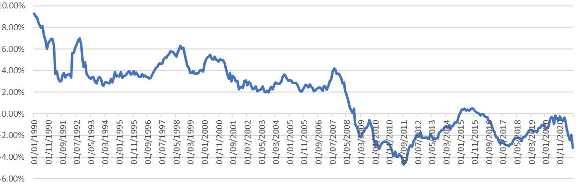
Line graph showing percentage values over time from January 1990 to January 2020, fluctuating between -4% and 9%.

Real return = annualised deposit rate – annual CPI (where deposit rate = Bank of England deposit rate from 31/01/2011 and weekly LIBOR prior to that)

Allowance for prudence

7.26Given inherent uncertainty in predicting the future and the limitations of our data and models, it may be appropriate to introduce a degree of prudence given that one can reduce contributions closer to retirement, but a shortfall discovered too late may be unbridgeable.

7.27It should also be borne in mind that the current environment is one in which funds will have particularly high 5-year volatilities, compared to historic averages. This introduces a mismatch between funds used to derive returns for particular volatility groups, and funds currently in those groups. This is most pertinent in the 0-5% volatility range but affects all groups. Therefore, a margin of prudence is particularly important in the present environment, to help mitigate the impact of this mismatch.

7.28In order to establish an appropriate level of prudence, the lower quartiles of returns for each volatility group were examined. Each fund-date pairing for which there is a 5-year volatility and subsequent return was considered an individual data point. The lower quartiles of all of these within each asset class was calculated. For consistency of comparison, the mean of the returns of funds within each category were recalculated. This included data for all month ends and hence yielded slightly different results from the previously derived mean returns:

Volatility Group	Volatility range	Mean return	Lower quartile	15-year returns Difference	Mean return	Lower quartile	10-year returns Difference
1	0%–0.5%	2.6%	1.9%	0.6%	1.9%	0.8%	1.1%
	0.5% - 2%	4.5%	3.1%	1.4%	2.9%	1.2%	1.7%
	2% - 5%	6.1%	5.3%	0.8%	6.3%	5.3%	1.0%
2	5% - 10%	6.8%	5.9%	0.9%	7.3%	6.2%	1.2%
3	10% - 15%	7.0%	5.7%	1.3%	8.1%	6.7%	1.4%
4	15% - 25%	8.8%	7.4%	1.3%	9.3%	7.6%	1.7%
	Over 25%	12.0%	10.7%	1.3%	9.5%	6.9%	2.6%

7.29The means and lower quartiles were calculated across all funds and all periods for which there is data. This therefore allows for both the possibility of a fund under-performing relative to the market, and the possibility of the market under-performing relative to other periods.

7.30The larger differences between the mean and quartile in the 0.5% - 2% level are mostly caused by the presence of some fixed income funds, which significantly bring up the mean return. Otherwise, we generally see the difference between mean and lower quartile increasing with volatility, especially for 10-year returns.

7.31The choice of a level of prudence will always be somewhat subjective. However, if an adjustment would leave an assumed rate close to the lower quartile of past returns, this may give us some confidence that the rate is still within reason while providing prudence.

7.32Based on the above rates table, an allowance of around 0.5% – 1% on expected returns for group 1 and 1% – 1.7% on expected returns for groups 2 to 4 do not seem unreasonable.

AS TM1 annual survey on the accumulation rate assumed by providers

7.33We also sought to gain insight from the return assumptions used by the current SMPI providers, based on the last AS TM1 survey conducted. Providers were asked to submit their return assumptions based on four asset classes: Equities, Corporate Bonds, Gilts, Cash. Within each asset class, there is likely a large amount of variation in term, nature and riskiness of the assets. The following shows the range of nominal returns assumed across the 17 providers who responded:

Asset class	AS TM1 annual survey accumulation rate assumption data Min	AS TM1 annual survey accumulation rate assumption data Average	AS TM1 annual survey accumulation rate assumption data Max
Equities	4.1%	5.5%	7.0%
Corporate Bonds	0.8%	2.4%	4.0%
Gilts	0.3%	0.8%	4.1%
Cash	0.5%	1.0%	1.5%

7.34The variation in the rates for the broad asset classes are understandably high. Providers may make assumptions at a much more granular level of asset classes, for example regions of equity figures or styles of equity funds could be treated separately. The figures providers submitted are likely to depend on the make-up of their portfolios. The progression of the returns from cash to gilts, then corporate bonds, then equities also varies greatly across the providers.

7.35AS TM1 has historically mandated a 7% cap for assumed accumulation rates until 2013 when the cap was removed and replaced with an annual survey to check the reasonableness of the assumptions made by providers. This may have influenced rates, and it is notable that the maximum return assumed is 7%.

Conclusion

7.36Taking into account all of the above, we set out in the table below how the proposed accumulation rate assumptions were determined. The assumptions are rounded to whole percentage figures to avoid spurious accuracy.

Group	Historical data analysis	Adjustment for bond effect	Adjustment for prudence	Implied rate	Accumulation rates assumptions
1	1.9%*		-1.0%	0.9%	1%
2	6.8%	-2%	-1.5%	3.3%	3%
3	7.1%	-0.5%	-1.5%	5.1%	5%
4	8.9%		-1.5%	7.4%	7%

Derived rate for the 0%–0.5% volatility range

7.37It is useful to understand how the accumulation rate assumptions above, if adopted, would compare to that used by providers based on the information from the last AS TM1 annual survey. The table below shows that accumulation rates assumptions are broadly within the range of the rates which current providers are assuming, whilst still somewhat higher than the average rates across the board.

Asset class	Expected volatility group to which this asset class will fall into	Implied accumulation rate (nominal)	AS TM1 annual survey accumulation rate assumption data Min	AS TM1 annual survey accumulation rate assumption data Average	AS TM1 annual survey accumulation rate assumption data Max
Equities	3 to 4	5%–7%	4.1%	5.5%	7.0%
Corporate Bonds	2 to 3	3%–5%	0.8%	2.4%	4.0%
Gilts	2	3%	0.3%	0.8%	4.1%
Cash	1	1%	0.5%	1.0%	1.5%

7.38We were also provided with assumptions used in various asset models in the marketplace privately. A comparison of the accumulation rate assumptions was made against the output of these asset models and we concluded that the accumulation rate assumptions were broadly consistent with output from the asset models in the market.

Appendix 1 – FRC's analysis of the external research

Independent academic research was conducted by Dr Paul Cox of the University of Bath to answer the following questions:
- Is there a relationship between DC fund investment risk and return?
- What is the relationship between the investment risk of a DC pension fund today and its future performance? What returns might be expected for a given level of risk?
- Is an SRRI categorisation a reasonable predictor of future returns?
Dr Cox's research is based on an enhanced data set. Typically, most individuals' pensions will be invested in a multi-asset fund of funds – meaning that they are effectively invested in a combination of the type of funds present in our data. Dr Cox created various combinations of the synthetic funds in the data to approximate these funds of funds, and focused his research on these.
The key findings we have drawn from Dr Cox's research to inform our own analysis are:
- There is an upward sloping relationship between 5-year risk taken and subsequent asynchronous (forward-looking) investment return. The further forward we project, the stronger that relationship becomes.
- Each additional 1% of risk taken appears to translate to an additional 0.3% – 0.4% of additional returns, based on a linear regression.
- The 7-level SRRI risk categorisation as it stands is limited in its usefulness as a proxy to estimated future returns:
- Multi-asset funds, which dominate the DC pension investments, fall mainly in SRRI category 4, with periods in category 5 according to economic conditions. This was demonstrated by measuring the volatility of a large number of synthetic multi-asset funds of funds, created using a bootstrapping methodology (randomly selecting funds from the population of single-asset funds in the data set according to a defined set of asset allocations).
- Volatility is time-varying, leading to periods when many funds have quantitatively high volatility and other periods when the same funds have quantitatively low volatility. That causes switching of categories not based on changes in forward investment returns.
- Market volatility, rather than a fund's beta, dominates the absolute value of volatility and any return projection.
- Given the concentration of DC funds in multi-asset default funds, a smaller number of risk categories may be appropriate.
- A relative measure of volatility based on the quantile of each fund relative to other funds has positive aspects including stability through varying economic conditions. However, there are clear practical limitations with a relative volatility measure since providers will not know their relative position within an acceptable timeframe.
- It was possible to partition the funds into two groups based on their relative volatilities, such that the subsequent returns were reliably higher in the higher risk group. However, partitioning them into three groups did not result in a significant difference in expected subsequent returns for all three groups.[^5]

Financial Reporting Council

8th Floor 125 London Wall London EC2Y 5AS +44 (0)20 7492 2300

www.frc.org.uk

[^1] Specifically, the annualised standard deviation of monthly returns over a 5-year period. [^2] Pearson and Spearman correlation coefficients both measure the strength of a correlation between two variables, with 1 indicating a perfect positive correlation, -1 indicating a perfect negative correlation, and 0 indicating no correlation. The Pearson indicates the strength of a linear relationship between the variables, whereas a Spearman coefficient is more appropriate for non-linear relationships. [^3] The SRRI methodology was developed as a way of giving investors a broad indication of the level of risk within an investment. It was developed in 2009 by a technical subgroup of the EU Committee of European Securities Regulators (CESR5) for use by UCITS in the Key Investor Information Document (KIID) and was consulted on and adopted by the EC6 in 2010. Fund volatility based on the latest 5 years' weekly price movements is used to assign UCITS portfolios into one of seven volatility (or risk) classifications. [^4] https://www.institutionalassetmanager.co.uk/2020/06/09/286348/forty-cent-ucits-share-classes-need-update-kiids-imminently [^5] It should be noted that the focus on synthetic multi-asset funds meant that the universe of funds Dr Cox was using existed almost entirely in the 5-15% volatility range. We do not therefore consider this result inconsistent with our proposal to use 4 volatility groups, which include groups of 0-5% and over 15%.

File

Name AS TM1 Accumulation Rates – Technical Analysis as at 31 August 2021

Publication date 27 September 2023

Format PDF, 2.3 MB

Download original

AS TM1 Accumulation Rates – Technical Analysis as at 31 August 2021

File

Is this page useful?